Observational studies often compare patients who received a treatment with patients who did not. However, these two groups usually differ before the treatment starts, and these differences can distort the results. Propensity score matching reduces this problem by creating groups of treated and untreated patients with similar baseline characteristics. A common mistake is to believe that propensity score matching removes all confounding, while it can only balance the variables that were measured. This guide explains the method in simple steps, using one hypothetical clinical example from the beginning to the end.
Table of Contents
What Is Propensity Score Matching?
The propensity score is the probability that a patient receives the treatment, given the patient’s measured baseline characteristics. It is usually estimated by logistic regression, and it summarizes many covariates in one number between 0 and 1. Propensity score matching then pairs each treated patient with an untreated patient who has a similar score (Austin, 2011). As a result, the matched groups can be compared in a way that resembles a randomized trial for the measured covariates.
Nearest Neighbor Matching
Each treated patient is matched to the untreated patient with the closest propensity score. This approach is simple. However, a poor match may be accepted when no similar untreated patient is available.
Caliper Matching
Caliper matching accepts a pair only when the two scores are within a pre-specified distance. A caliper of 0.2 of the standard deviation of the logit of the propensity score is widely recommended (Austin, 2011).
Optimal and Full Matching
Optimal matching minimizes the total distance across all pairs, instead of selecting the closest match one patient at a time. Full matching forms matched sets that use all eligible patients (Stuart, 2010).
Importance of Propensity Score Matching in Medical Research
Reducing Confounding by Indication
Physicians do not assign treatments at random. For example, healthier patients may be more likely to receive an intensive program. Propensity score matching reduces the bias produced by these measured differences.
Separating Design from Outcome Analysis
The matching can be completed before the outcome is examined. Therefore, the researcher can check the balance of covariates without being influenced by the treatment effect.
Presenting Balance Transparently
A balance table shows readers whether the matched groups are comparable. This table is easier to understand than the adjustment performed inside a multivariable model.
Applications of Propensity Score Matching in Clinical Studies
Comparative Effectiveness Studies
When a randomized trial is unethical or impractical, propensity score matching is used to compare treatments in registries and cohort studies, such as two surgical techniques.
Drug Safety Research
Rare adverse events are often studied in large electronic health records. Matching on propensity scores helps researchers compare new users of a drug with similar users of another drug.
Studies with Time-to-Event Outcomes
Matched samples are also used with survival outcomes. In this situation, the matched data are commonly analyzed with Cox proportional hazard analysis.
Assumptions of Propensity Score Matching
Before applying the method, the following assumptions must be considered:
- No unmeasured confounding: all variables that affect both treatment assignment and the outcome have been measured. This is the crucial assumption, and it cannot be proven from the data.
- Overlap (positivity): every patient has a probability of receiving treatment above 0 and below 1, so comparable patients exist in both groups.
- Baseline covariates only: the variables in the model are measured before the treatment and are not affected by it.
- Correct propensity score model: the model includes the relevant confounders and achieves balance in the matched sample.
- Adequate sample size: enough untreated patients are available to provide good matches. You can read more in our guide on sample size in research.
How to Perform Propensity Score Matching: A Clinical Example
Consider a hypothetical retrospective cohort of 1,000 patients after acute myocardial infarction. A total of 400 patients attended cardiac rehabilitation, and 600 did not. The outcome was hospital readmission within one year. The data were simulated for teaching purposes, and every value below was calculated from this simulated dataset.
Step 1: Define the Research Question and the Confounders
The question is: does cardiac rehabilitation reduce one-year readmission? Before the analysis, five baseline confounders were selected based on clinical knowledge: age, female sex, diabetes, current smoking, and left ventricular ejection fraction (LVEF).
Step 2: Examine the Baseline Imbalance
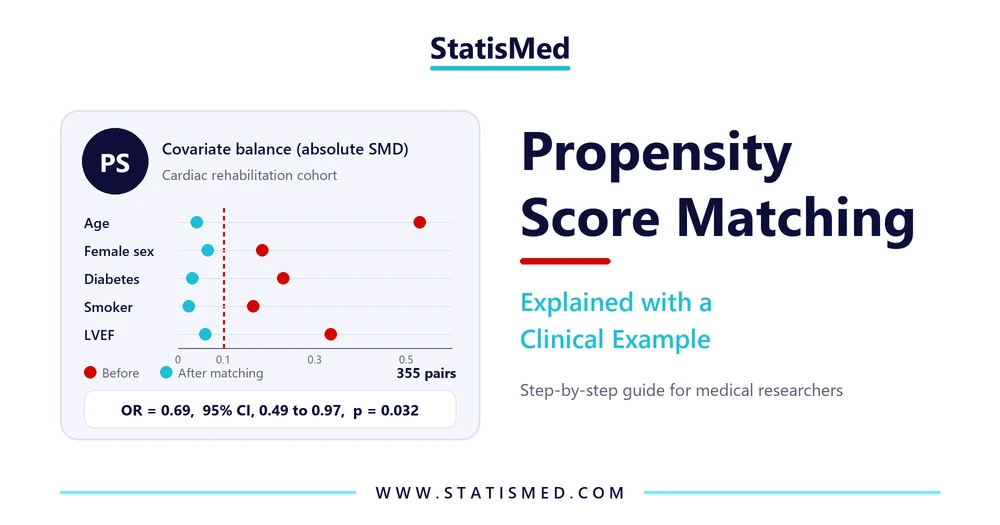
The standardized mean difference (SMD) compares groups independently of the sample size. For age, SMD = (58.9 − 64.3) ÷ √[(9.9² + 10.5²) ÷ 2] = −0.529. An absolute SMD below 0.1 is commonly taken to indicate a negligible difference (Austin, 2011). The groups were clearly imbalanced before matching, since rehabilitation attendees were younger and healthier:
| Covariate | Rehabilitation (n = 400) | No rehabilitation (n = 600) | Absolute SMD |
|---|---|---|---|
| Age, mean ± SD | 58.9 ± 9.9 | 64.3 ± 10.5 | 0.529 |
| Female sex | 98 (24.5%) | 197 (32.8%) | 0.185 |
| Diabetes | 101 (25.3%) | 215 (35.8%) | 0.231 |
| Current smoker | 131 (32.8%) | 244 (40.7%) | 0.165 |
| LVEF (%), mean ± SD | 51.8 ± 8.7 | 48.9 ± 8.6 | 0.334 |
Before matching, readmission occurred in 23.3% of attendees and 37.7% of non-attendees (χ² = 22.96, df = 1, p < 0.001; OR = 0.50, 95% CI, 0.38 to 0.67). This comparison was calculated with the chi-square test, and it is confounded by the differences above.
Step 3: Estimate the Propensity Score
A logistic regression model was fitted with rehabilitation attendance as the dependent variable and the five confounders as predictors. The outcome is not included in this model.
| Covariate | β | OR | 95% CI | p-value |
|---|---|---|---|---|
| Intercept | 1.3159 | |||
| Age (per year) | −0.0562 | 0.95 | 0.93 to 0.96 | < 0.001 |
| Female sex | −0.4403 | 0.64 | 0.48 to 0.87 | 0.004 |
| Diabetes | −0.6221 | 0.54 | 0.40 to 0.73 | < 0.001 |
| Current smoker | −0.4459 | 0.64 | 0.48 to 0.85 | 0.002 |
| LVEF (per 1%) | 0.0439 | 1.04 | 1.03 to 1.06 | < 0.001 |
For a 60-year-old non-smoking man with diabetes and LVEF of 50%, the logit equals 1.3159 − 0.0562(60) − 0.6221 + 0.0439(50) = −0.483. Therefore, the propensity score equals e−0.483 ÷ (1 + e−0.483) = 0.38.
Step 4: Check the Overlap of Propensity Scores
Propensity scores ranged from 0.076 to 0.873 among attendees and from 0.045 to 0.806 among non-attendees. The distributions overlapped widely, so matching was feasible. In practice, overlap is best examined with a histogram or density plot of the scores in each group.
Step 5: Match the Patients
We used 1:1 nearest neighbor matching without replacement, starting from the highest score. The caliper was 0.2 × 0.809 = 0.162 on the logit scale. Propensity score matching produced 355 pairs. Consequently, 45 attendees (11.3%) had no acceptable match, and 245 non-attendees remained unused.
Step 6: Re-Check the Balance After Matching
Balance should be assessed in the matched sample using the SMD. Notably, significance testing is discouraged for this purpose (Austin, 2011). All absolute SMDs became lower than 0.1:
| Covariate | Rehabilitation (n = 355) | No rehabilitation (n = 355) | SMD before | SMD after |
|---|---|---|---|---|
| Age, mean ± SD | 60.2 ± 9.4 | 60.6 ± 9.6 | 0.529 | 0.041 |
| Female sex | 93 (26.2%) | 83 (23.4%) | 0.185 | 0.065 |
| Diabetes | 96 (27.0%) | 101 (28.5%) | 0.231 | 0.031 |
| Current smoker | 123 (34.6%) | 127 (35.8%) | 0.165 | 0.024 |
| LVEF (%), mean ± SD | 51.0 ± 8.5 | 50.5 ± 8.6 | 0.334 | 0.060 |
Step 7: Estimate the Treatment Effect in the Matched Sample
The two patients in a pair are not independent, so the analysis should account for matching (Austin, 2011). For a binary outcome, McNemar’s test is suitable, and it uses the discordant pairs:
| Matched pairs (n = 355) | Control readmitted | Control not readmitted |
|---|---|---|
| Rehabilitation patient readmitted | 32 | 55 |
| Rehabilitation patient not readmitted | 80 | 188 |
Readmission occurred in 87 attendees (24.5%) and 112 matched non-attendees (31.5%). McNemar’s χ² = (55 − 80)² ÷ (55 + 80) = 4.63, df = 1, p = 0.031. With continuity correction, χ² = 4.27 and p = 0.039, which leads to the same conclusion. The matched odds ratio equals 55 ÷ 80 = 0.69 (95% CI, 0.49 to 0.97), and the risk difference equals −7.0 percentage points (95% CI, −13.4 to −0.7). Our guides on confidence intervals and effect size explain these estimates further.
Importantly, the risk difference decreased from −14.4 percentage points before matching to −7.0 after matching. Part of the crude difference was therefore explained by measured confounders.
How to Report Propensity Score Matching Results in a Manuscript
The Methods section should state the covariates, the matching ratio, the caliper, and the balance criterion. The Results section should present the matched sample size, balance, and the treatment effect, as shown below:
One-Year Readmission After Propensity Score Matching
A total of 355 matched pairs were created from 1,000 patients, and all absolute standardized mean differences were below 0.1 after matching. One-year readmission was significantly lower among patients who attended cardiac rehabilitation (24.5%) compared to those who did not attend (31.5%) (McNemar χ² = 4.63, df = 1, p = 0.031). Moreover, attendance was associated with lower odds of readmission (OR = 0.69, 95% CI, 0.49 to 0.97, p = 0.032). (Table 3)
Notably, possible explanations of the association and comparisons with previous studies belong to the Discussion section, not to the Results.
Common Mistakes When Using Propensity Score Matching
Assuming That Matching Solves Unmeasured Confounding
Propensity score matching balances measured variables only. Therefore, unmeasured factors, such as patient motivation, can still bias the estimate. A sensitivity analysis should be considered.
Including Post-Treatment Variables
Variables measured after treatment may be affected by the treatment. Including them can introduce bias, so only pre-treatment covariates should enter the model.
Using P-Values or the C-Statistic to Judge Balance
The c-statistic describes how well the model discriminates between treated and untreated patients. However, it does not show whether the propensity score model is correctly specified (Austin, 2011). Balance must be checked directly using the SMD.
Ignoring the Pairing in the Final Analysis
Analyzing a matched sample with independent-sample tests ignores the lack of independence. Instead, McNemar’s test or a paired t-test should be used, depending on the outcome.
Ignoring the Excluded Patients
Patients without a match are removed from the analysis, so the result applies to the matched population. Researchers should report how many patients were excluded and compare their characteristics.
Running Propensity Score Matching in SPSS and R
In SPSS, propensity score matching is usually performed with a free extension. First, install the PSM and FUZZY extensions through Extensions → Extension Hub. Then choose Data → Propensity Score Matching, specify the treatment group indicator and the covariates, and set the match tolerance. This dialog creates one-to-one matches. In R, the MatchIt package performs the same analysis with one line of code: matchit(rehab ~ age + female + diabetes + smoker + lvef, data = d, method = "nearest", distance = "glm", link = "linear.logit", caliper = 0.2). For retrospective designs, you can also read our guide on case-control studies.
Conclusion
Propensity score matching is a transparent method for reducing measured confounding in observational studies. Correct use requires clinically selected baseline covariates, adequate overlap, balance assessment with the SMD, and an analysis that accounts for the pairs. If you need support in designing your matching strategy, analyzing your data, or writing your Results section, the StatisMed team of biostatisticians provides statistical analysis services for medical studies. You can request a free quote today.
Frequently Asked Questions
1. Is propensity score matching better than multivariable regression?
Neither method is always better. Both rely on measured confounders. However, propensity score matching makes balance easy to inspect, and it is useful when there are few outcome events and many covariates.
2. Which matching ratio should I use?
The 1:1 ratio is the most common and produces close matches. A higher ratio, such as 1:2, can retain more patients when many untreated patients are available, but the additional matches may be less similar.
3. What should I do if the SMD remains above 0.1 after matching?
Revise the propensity score model, for example by adding interaction or quadratic terms, or use a narrower caliper. Then re-check the balance. The outcome should not be used to choose among the models.
References
Austin, P. C. (2011). An introduction to propensity score methods for reducing the effects of confounding in observational studies. Multivariate Behavioral Research, 46(3), 399–424. https://doi.org/10.1080/00273171.2011.568786
Stuart, E. A. (2010). Matching methods for causal inference: A review and a look forward. Statistical Science, 25(1), 1–21. https://doi.org/10.1214/09-STS313