
Medical researchers often need to know whether the distribution of a categorical variable in their sample matches a known or expected distribution. For example, does the distribution of blood groups among patients with a disease match that of the general population? The goodness of fit test answers this question. It compares the observed counts in each category with the counts expected under a stated hypothesis. A common mistake is to confuse the goodness of fit test with the chi-square test of independence, which compares two variables rather than one. This guide explains the chi-square goodness of fit test step by step, using one hypothetical clinical example.
Table of Contents
Free tool: calculate the sample size or power for your study with the StatisMed sample size calculator. It shows the exact R code and ready-to-use wording for your Methods section. Open the calculator →
What Is a Goodness of Fit Test?
A goodness of fit test examines how well observed data agree with a theoretical or reference distribution. The most widely used version in medical research is the chi-square goodness of fit test, which belongs to the same family as the chi-square test of independence. Both tests are based on the difference between observed and expected frequencies (McHugh, 2013).
Chi-Square Goodness of Fit Test
This test is used with one categorical variable that has two or more categories, such as blood group, disease stage, or day of hospital admission. The expected counts come from the null hypothesis, which may state equal proportions in all categories or specific proportions from a reference population, a previous study, or a genetic model.
Goodness of Fit Tests for Continuous Data
For continuous variables, other goodness-of-fit tests are used. The Kolmogorov-Smirnov and Shapiro-Wilk tests, for example, check whether data follow a normal distribution. These tests follow the same logic, but they work on the shape of a continuous distribution rather than on counts.
Goodness of Fit for Statistical Models
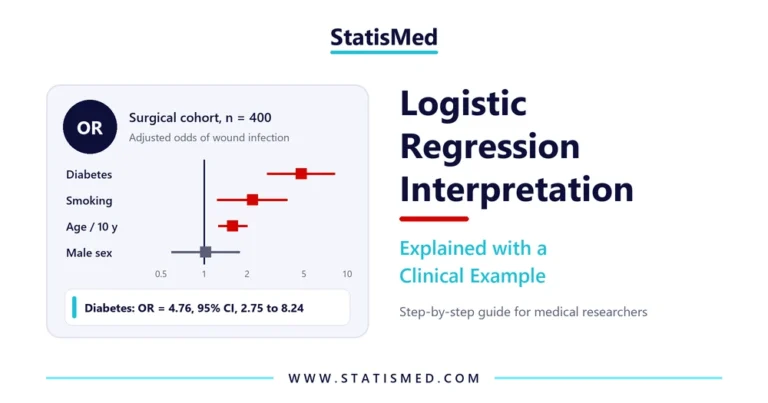
The term is also used for regression models. The Hosmer-Lemeshow test, for instance, checks whether the probabilities predicted by a logistic model agree with the observed outcomes (see logistic regression interpretation). In this guide, however, the focus is on the chi-square goodness of fit test for categorical data.
Importance of the Goodness of Fit Test in Medical Research
Comparison with a Reference Population
Many clinical questions start with a comparison between a patient group and the general population. The goodness of fit test shows whether a disease group has an unusual distribution of a characteristic, such as blood group, sex, or ethnicity.
Checking the Representativeness of a Sample
Before generalizing results, researchers need to know whether the sample resembles the target population. Therefore, the test is often used to compare the age or sex distribution of a sample with census data.
Testing Genetic and Theoretical Models
In genetic studies, the test checks whether genotype frequencies follow the Hardy-Weinberg equilibrium. Moreover, it can test whether events, such as hospital admissions, are evenly distributed across days or months.
Applications of the Goodness of Fit Test in Clinical Studies
Clinical Trials
In randomized trials with unequal allocation, such as 2:1, the test can check whether the achieved allocation agrees with the planned ratio. It can also compare the distribution of baseline categories with the trial’s eligibility population.
Epidemiological Studies
Epidemiologists use the goodness of fit test to compare the distribution of cases by season, region, or age group with the distribution expected from population data. A significant result may point to clustering or to a risk factor that needs further study.
Surveys and Quality Audits
In surveys, the test shows whether responses are evenly spread across options or whether the respondents’ profile matches the sampling frame. In hospital audits, it can compare the distribution of complications with a national benchmark.
Assumptions of the Chi-Square Goodness of Fit Test
Before running the test, check that the data meet the following assumptions (Kim, 2017):
- The variable is categorical (nominal or ordinal), and the data are counts, not percentages or means.
- Each participant contributes to one category only, and the observations are independent.
- The categories are mutually exclusive and together include all participants.
- The expected proportions are specified before looking at the data.
- The expected frequency is at least 5 in each category (or in at least 80% of categories, with none below 1).
If the expected counts are too small, categories can be combined in a meaningful way. With only two categories and small counts, an exact binomial test is preferred.
How to Perform a Goodness of Fit Test: A Clinical Example
Consider a hypothetical study of 300 patients with gastric cancer. The researchers want to know whether the distribution of ABO blood groups among these patients differs from the distribution in the general population. For this example, assume that the reference distribution is O 45%, A 40%, B 11%, and AB 4%. All the numbers below were calculated with Python.
Step 1: State the Hypotheses
The null hypothesis (H0) states that the blood group distribution among the patients is the same as the reference distribution. The alternative hypothesis (H1) states that the distribution differs from the reference distribution in at least one category. The significance level is set at 0.05.
Step 2: Record the Observed Counts
Among the 300 patients, 110 had blood group O, 140 had A, 36 had B, and 14 had AB. These observed counts (O) are shown in Table 1 together with their percentages.
Step 3: Calculate the Expected Counts
The expected count (E) for each category equals the total sample size multiplied by the expected proportion. For blood group O, E = 300 × 0.45 = 135. In the same way, the expected counts are 120 for A, 33 for B, and 12 for AB.
| Blood group | Observed n (%) | Expected proportion | Expected n |
|---|---|---|---|
| O | 110 (36.7%) | 0.45 | 135 |
| A | 140 (46.7%) | 0.40 | 120 |
| B | 36 (12.0%) | 0.11 | 33 |
| AB | 14 (4.7%) | 0.04 | 12 |
| Total | 300 (100%) | 1.00 | 300 |
Step 4: Check the Expected Frequencies
The smallest expected count is 12 (blood group AB). Since all expected counts are above 5, the chi-square approximation is valid, and no categories need to be combined.
Step 5: Calculate the Chi-Square Statistic
The test statistic is χ² = Σ (O − E)² ÷ E, summed over all categories. Table 2 shows the contribution of each blood group. Notably, blood group O contributes more than half of the total value.
| Blood group | O | E | O − E | (O − E)² | (O − E)² ÷ E |
|---|---|---|---|---|---|
| O | 110 | 135 | −25 | 625 | 4.630 |
| A | 140 | 120 | 20 | 400 | 3.333 |
| B | 36 | 33 | 3 | 9 | 0.273 |
| AB | 14 | 12 | 2 | 4 | 0.333 |
| Total | 300 | 300 | 0 | χ² = 8.57 |
Step 6: Find the Degrees of Freedom and the P-Value
The degrees of freedom equal the number of categories minus 1, so df = 4 − 1 = 3. The critical value of chi-square at df = 3 and α = 0.05 is 7.81. Because the calculated value (8.57) is larger than 7.81, the null hypothesis is rejected. The exact p-value is 0.036 (χ² = 8.57, df = 3, p = 0.036).
Step 7: Calculate the Effect Size and the Residuals
A p-value does not show how large the departure is. Therefore, report an effect size, such as Cohen’s w = √(χ² ÷ n) = √(8.57 ÷ 300) = 0.17. By Cohen’s benchmarks (0.10 small, 0.30 medium, 0.50 large), this is a small effect.
A significant goodness of fit test also does not show which categories differ. For this purpose, calculate the adjusted standardized residual for each category: (O − E) ÷ √[E × (1 − p)], where p is the expected proportion. Values beyond ±1.96 indicate a category that departs from expectation at the 0.05 level. Because four categories are tested, a Bonferroni correction (0.05 ÷ 4 = 0.0125) protects against false positive findings.
| Blood group | Adjusted residual | p-value | Bonferroni-adjusted p |
|---|---|---|---|
| O | −2.90 | 0.004 | 0.015 |
| A | 2.36 | 0.018 | 0.074 |
| B | 0.55 | 0.580 | 1.000 |
| AB | 0.59 | 0.556 | 1.000 |
Blood group O was less frequent than expected, and this difference remained significant after the Bonferroni correction. In contrast, the excess of blood group A was significant before correction only.
How to Report Goodness of Fit Test Results in a Manuscript
In the Methods section, state the test, the source of the expected proportions, and the software. For example: “The chi-square goodness of fit test was used to compare the ABO distribution with the reference population distribution.” In the Results section, report the significant findings only, as in the model paragraph below.
ABO Blood Group Distribution Among Patients with Gastric Cancer
The distribution of ABO blood groups among the 300 patients differed significantly from the reference population distribution (χ² = 8.57, df = 3, p = 0.036, Cohen’s w = 0.17). Blood group O was significantly less frequent than expected (36.7% vs 45.0%, adjusted residual = −2.90, Bonferroni-adjusted p = 0.015) (Table 1).
Notice that the paragraph gives the numbers without any explanation of why the difference exists. The interpretation and the comparison with previous studies belong in the Discussion section.
Common Mistakes When Using the Goodness of Fit Test
Using Percentages Instead of Counts
The chi-square statistic must be calculated from actual counts. Entering percentages gives a wrong value, because the result depends on the sample size. For instance, 36.7% of 300 and 36.7% of 30 carry very different amounts of information.
Choosing the Expected Proportions After Seeing the Data
The expected distribution must come from an external source, such as census data or a published study, and must be defined in the protocol. Selecting the reference after seeing the data inflates the chance of a significant result.
Confusing It with the Test of Independence
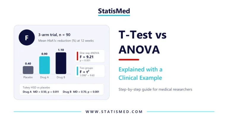
The goodness of fit test has one variable and a fixed expected distribution. In contrast, the test of independence has two variables, and the expected counts come from the row and column totals. Our guide to choosing the right statistical test explains this difference further.
Interpreting a Non-Significant Result as Proof of Fit
A non-significant goodness of fit test does not prove that the sample follows the reference distribution. In small samples, the test has low power. Therefore, plan an adequate sample size before the study.
Ignoring Small Expected Counts
When expected counts are below 5, the p-value from the chi-square distribution may be inaccurate. In this case, combine sparse categories or use an exact multinomial test, similar to the use of Fisher’s exact test for small 2×2 tables.
Running the Goodness of Fit Test in SPSS and R
In SPSS, the test is performed through Analyze → Nonparametric Tests → Legacy Dialogs → Chi-square. Move the blood group variable to “Test Variable List”. Under “Expected Values”, select “Values” and add the expected proportions (45, 40, 11, 4) in the same order as the category codes. SPSS reports the observed and expected counts, the residuals, the chi-square value, df, and the p-value. In R, the same analysis is performed with one line of code: chisq.test(x = c(110, 140, 36, 14), p = c(0.45, 0.40, 0.11, 0.04)). The adjusted residuals are available from the stdres element of the result.
Conclusion
The chi-square goodness of fit test is a simple method to compare the distribution of one categorical variable with an expected distribution. Correct use requires counts, independent observations, expected proportions defined in advance, and adequate expected frequencies. Moreover, a complete report includes the chi-square value, df, the p-value, an effect size, and the categories that differ. If you need support in selecting the appropriate test, analyzing your data, or writing the Results section of your manuscript, the StatisMed team of biostatisticians provides statistical analysis services for medical studies. You can request a free quote today.
Frequently Asked Questions
1. What is the difference between the goodness of fit test and the chi-square test of independence?
The goodness of fit test compares one categorical variable with a known or hypothesized distribution. The test of independence examines whether two categorical variables are associated in a contingency table. Both use the same chi-square formula, but the expected counts are calculated differently.
2. How are the degrees of freedom calculated for a goodness of fit test?
The degrees of freedom equal the number of categories minus 1. If parameters of the expected distribution are estimated from the same data, one additional degree of freedom is subtracted for each estimated parameter.
3. Can I use the goodness of fit test with only two categories?
Yes. With two categories, the test has df = 1 and gives the same result as the large-sample binomial test of one proportion. When the sample is small, the exact binomial test is the better choice.
References
Kim, H. Y. (2017). Statistical notes for clinical researchers: Chi-squared test and Fisher’s exact test. Restorative Dentistry & Endodontics, 42(2), 152–155. https://doi.org/10.5395/rde.2017.42.2.152
McHugh, M. L. (2013). The chi-square test of independence. Biochemia Medica, 23(2), 143–149. https://doi.org/10.11613/BM.2013.018